4.  Modal Sublimation: How the Possible Becomes Real

Water does not get steadily more solid as it cools. At zero degrees it becomes ice, all at once. This chapter argues the substrate does something similar: when the leftover pull passes a certain size, a configuration stops being merely possible and becomes real. That sudden change is what the book calls modal sublimation.

This chapter develops P3, modal sublimation. Where P1 supplies primitive distinguishability and P2 supplies its asymmetric tension, P3 supplies the transition mechanism: a Landau–Ginzburg threshold beyond which the uninstantiated substrate cannot maintain itself, producing instantiated geometry along the substrate’s net direction. The chapter has two parts: the threshold mechanism that drives the transition (§4.1 and following) and the sublimation transition itself, formalised as a categorical functor and constructed explicitly.

4.1.  Why a modal threshold must exist

The existence of asymmetric tension raises an immediate question: if differentiated configurations carry a structural imbalance, what prevents the substrate from containing arbitrarily large imbalances indefinitely? The answer given by PST is that the substrate is not unlimited in this respect. There is a boundary to what can remain uninstantiated, one that is not physical, not dynamical, and not temporal, but purely logical. (This boundary is modal: a logical and structural bound on uninstantiated imbalance, the modal threshold $\tau$. It is not a spatial or cosmological bound on the size or finitude of the universe. That separate question is addressed in §1.7 via the emergent topology $M=\mathbb{R}\times S^{3}$.)

To understand why this boundary must exist, recall the character of the precausal substrate. It is a domain that is defined entirely by what can be coherently maintained without spacetime, without causal structure, and without any form of realisation. A configuration exists in the substrate insofar as it is a coherent arrangement of distinctions: its properties are differentiated from one another, and that differentiation constitutes its identity. Coherence here is not a quantitative threshold in the ordinary sense. It is a modal condition: a configuration is coherent as an uninstantiated structure if and only if it can exist as such without contradiction.

Now, asymmetric tension is the imbalance inherent in any differentiated configuration. As the number and depth of distinctions within a configuration increase, the magnitude $|T(C)|=\sqrt{\langle T(C),T(C)\rangle}$ of its $V_{7}$-valued asymmetric tension increases. This monotonicity is not derivable from the axioms of $(D,\delta,v)$ alone; it is a structural constraint on $T$ that PST adopts as part of its encoding. Three structural constraints on $T$ are required:

$$|T(C)| \;\geq\;0,\quad|T(C)|=0\;\Leftrightarrow\;C\text{ has no distinct pairs}$$ (14)

$$|T(C\cup\{a\})| \;\geq\;|T(C)|\quad\forall\,a\notin C$$ (15)

$$T(\bar{C}) \;\neq\;-T(C)\quad\text{generically}$$ (16)

Equation (14) is magnitude positivity, equation (15) is magnitude monotonicity, and equation (16) is complement vector asymmetry. The last says that the substrate’s total tension $T(D)$, the tension of the maximal configuration $C=D$, is generically a nonzero $V_{7}$-vector, providing the substrate-level directional bias $\hat{\tau}$ that P2 names. Generically rather than necessarily: the two constraints do not establish the same thing. (14) forces the magnitude $|T(D)|>0$, since $D$ contains distinct pairs, whereas the $V_{7}$-vector $T(D)$ is nonzero only where the elementary directions fail to cancel antipodally. That non-balance is independent of (14), and it is unforced: an open condition with a sharp margin, a stability statement rather than a probabilistic one (§3.4, Computation 152). The magnitude constraints (14)–(15) and the directional constraint (16) bear on different aspects of $T$, its scalar magnitude and its $V_{7}$-direction. A minimal example for the magnitude structure is the induced edge count:

$$T_{\mathrm{ex}}(C)\;=\;\bigl{|}\bigl{\{}(a,b)\;:\;a,b\in C,\;a\neq b,\;\delta(a,b)\bigr{\}}\bigr{|}$$ (17)

Equation (14) holds for any configuration with at least two distinct properties. Equation (15) holds by inspection: adding property $a$ to $C$ increases the count by $|\{b\in C:\delta(a,b)\}|$. At the scalar (magnitude) level, the analogue of (16) (that $T_{\mathrm{ex}}(C)\neq T_{\mathrm{ex}}(\bar{C})$) holds whenever the induced subgraphs on $C$ and $\bar{C}$ have different edge counts, generic for non-regular distinction structures. Equations (14)–(16) do not rule out regular distinction graphs; for a regular $(D,\delta)$ the induced subgraphs on complementary subsets of equal size can share the same edge count, so $T_{\mathrm{ex}}$ fails complement-asymmetry there. The example therefore satisfies the constraints on a generic, not universal, sub-class of $(D,\delta)$. This scalar example fixes the magnitude but carries no $V_{7}$-direction; the directional content comes from aggregating the elementary directions $v(a)$ that P1 assigns. The random-walk form $T(C)=\sum_{a\in C}v(a)$, with $v(a)\in V_{7}$ unit vectors, models that directional aggregation and is the tractable model used in the large-deviation analysis of Computation 75. Neither is the unique form of $T$; an admissible $T$ pairs a magnitude satisfying (14)–(15) with a $v$-inherited $V_{7}$-direction, and its precise form is contingent rather than derived from P1–P3 (§14.3).

The underdetermination this leaves is precise, and bounded. Constrained only by (14)–(15), the magnitude ranges over a family whose dimension grows as $2^{|D|}$. Any order-preserving function on the configuration lattice that vanishes exactly on the distinction-free configurations is admissible, with $T_{\mathrm{ex}}$ one representative among them, so the form is not a finite-parameter object (Computation 126). What the constraints fix is not a form but three structural facts: the codomain, $T$ being $V_{7}$-valued as forced by the Hurwitz constraint in P1; the magnitude’s zero locus (14); and the existence of a nonzero global bias $T(D)$, hence a well-defined direction $\hat{\tau}$ (16). Almost every later derivation reads $T$ through only two of these: the ordering of the magnitudes $|T(C)|$, which is what the threshold dynamics of the following chapters require, and the single global direction $\hat{\tau}=T(D)/|T(D)|$; no result uses the direction of $T(C)$ at any non-maximal configuration. One derivation is not of that kind and must be named: the Born-consistency comparison (98) tests $\tau_{0}(C)$ against Born weights carrying their own normalisation, which is a cardinal read and not an ordinal one (§10.3.2.5). The remaining freedom is therefore confined to exactly the per-configuration content that §14.3 reads as contingent input, which leaves the structural skeleton the rest of this work relies on fully fixed. Computation 140 verifies that robustness by exhibiting the exact invariance under which the instantiation sequence, the per-configuration phase, and the bias direction are all unchanged: monotone reparametrisation of the magnitudes with $\hat{\tau}$ fixed. The one cardinal read holds for the realised content as well, since P3’s typicality reaches that content (§1.7, Computations 193, 195), so the conclusion holds in full: only the ordering of the magnitudes and $\hat{\tau}$ are load-bearing, and the canonical form of $T(C)$ is a bounded underdetermination that is no longer carried on the structural front (Appendix C).

A modest imbalance can be sustained within the substrate without contradiction, just as a small asymmetry in a logical structure does not render it incoherent. But there is a limit. At some critical level of imbalance, the structural pressure accumulated within the configuration is such that remaining uninstantiated would require holding together a structure whose internal tension actively resists the very absence of a resolving medium. There is no geometry, no dynamics, no causal channel through which the imbalance could redistribute. The configuration carries more structural demand than uninstantiated existence can absorb.

This is the modal threshold. It is the limit on the modal coherence of uninstantiated structure: beyond a certain level of asymmetric tension, a configuration can no longer be maintained within the precausal, nonspatiotemporal domain. Its structural incoherence has reached the point at which remaining uninstantiated is no longer a modally coherent option. The configuration has not been acted upon by anything. No force has been applied and no event has occurred. It is simply that continued uninstantiated existence has become logically excluded.

The threshold is therefore a logical boundary condition: a constraint on what is modally possible in the precausal substrate, analogous to the logical impossibility of a contradiction rather than to a physical limit imposed by dynamics. This analogy is worth dwelling on. When a contradiction is derived in a formal system, it does not occur at a specific time and it is not caused by any preceding state. It is simply that the set of propositions in question cannot all be simultaneously true. The modal threshold is the ontological counterpart: a configuration whose tension exceeds $\tau$ cannot simultaneously be differentiated to that degree and remain uninstantiated. The two are incompatible modes of being, and incompatibility is not a causal relation but a logical one.

4.2.  The boundary condition on $|T(C)|$

The modal threshold is formalised as follows. There exists a critical value $\tau\in\mathbb{R}^{+}$ such that:

$$|T(C)|\geq\tau\;\implies\;C\text{ cannot remain uninstantiated}$$ (18)

Several features of this implication deserve comment. First, it is a one-way entailment: exceeding $\tau$ necessitates instantiation, but there is no corresponding claim that every instantiated configuration arrived at that state by exceeding $\tau$ from a specific prior configuration. The precausal substrate is not temporal; configurations do not “arrive” at tension values through a sequence of states. The implication holds modally, not temporally.

Second, the implication expresses modal necessity, not causal consequence. It does not say that something happens to a configuration when $T(C)\geq\tau$. It says that the mode of being characterised by uninstantiated existence is not available to such a configuration. The language of “cannot remain” is a concession to ordinary usage; strictly, the configuration was never coherently uninstantiated once its tension reached that level.

Third, the value $\tau$ is not a free parameter of the theory. It cannot be chosen arbitrarily or tuned to match observations. As the variational treatment below makes clear, $\tau$ is the unique value at which the modal structure of the substrate changes its minimal configuration from uninstantiated to instantiated. It is derived from the structure of the functional, not imposed from outside.

To quantify how far a given configuration sits above the threshold, define the excess tension:

$$\varepsilon(C)\;=\;|T(C)|-\tau$$ (19)

For configurations below the threshold, $\varepsilon(C)<0$ and uninstantiated existence remains coherent. For configurations above the threshold, $\varepsilon(C)>0$ and instantiation is necessitated. Configurations with $\varepsilon(C)=0$ inhabit the threshold precisely: they sit at the boundary of modal coherence, neither firmly in the uninstantiated regime nor fully instantiated. It is these marginal configurations that exhibit the most delicate modal behaviour. As shown in Chapter 10, they are the configurations that give rise to the phenomena of quantum mechanics: the indeterminacy, the superposition, and the probabilistic character of quantum measurement all arise from the modal ambiguity of configurations at exactly $\varepsilon=0$.

The parameter $\varepsilon$ will serve as the primary variable throughout the remainder of the book. It measures not tension in absolute terms but tension relative to the threshold, and it is this relative measure that determines which mode of being a configuration occupies.

4.3.  The order parameter and its ontological status

To derive $\tau$ from first principles, it is necessary to introduce a quantity that tracks the transition between uninstantiated and instantiated existence continuously. In the theory of phase transitions, such a quantity is called an order parameter: a scalar field that is zero in one phase and nonzero in the other, and whose value characterises how deep into the new phase the system has penetrated. PST introduces an analogous quantity for the modal transition.

Define $\psi(C)\in V_{7}$ as the modal order parameter: a $V_{7}$-valued field over configuration space encoding the modal status of each configuration. The value $\psi=0$ denotes the uninstantiated phase. Nonzero values of the magnitude $|\psi|=\sqrt{\langle\psi,\psi\rangle}$ indicate degrees of instantiation, with larger $|\psi|$ corresponding to deeper settlement into the instantiated vacuum. The unit direction $\hat{\psi}=\psi/|\psi|$ on $S^{6}\subset V_{7}$ carries the directional content of the instantiation event. The $V_{7}$-valued representation inherits from the directional content of P1: an order parameter for asymmetric vector tension must take values in the same direction algebra.

The full $G_{2}$ symmetry of $V_{7}$ (rotations preserving the inner product and the vector product) is the symmetry under which the modal potential is invariant; the $\mathbb{Z}_{2}$ symmetry $\psi\to-\psi$ is the antipodal involution on $S^{6}$, a $G_{2}$-equivariant special case. Each of the $S^{6}$ directions is a candidate “which way” the vacuum will settle; modal sublimation locks $\hat{\psi}$ to the substrate’s net direction $\hat{\tau}=T(D)/|T(D)|$ (P2).

The ontological status of $\psi$ requires careful handling. In condensed matter physics, an order parameter such as magnetisation has a clear physical meaning: it is the average magnetic moment per unit volume, measurable in principle at every point in space at every time. The modal order parameter $\psi$ is not measurable in this sense. It is not a field over spacetime, because spacetime does not exist until after the transition. It is instead a field over configuration space $\mathcal{C}$, taking values in $V_{7}$: it assigns to each precausal configuration a $V_{7}$-vector that encodes its modal status. This is not a physical field; it is a structural characterisation of the substrate. Its role is formal: it provides the mathematical language needed to locate the threshold magnitude $\tau$ and the substrate-determined direction $\hat{\tau}$ from the structure of the modal potential.

4.4.  Variational formulation of $\tau$

With the order parameter in hand, $\tau$ can be derived from a variational principle rather than assumed. The strategy is to write down the simplest functional $\mathcal{F}[\psi]$ over configuration space whose structure is fully determined by two requirements: it must be consistent with the symmetries of the substrate, and it must be capable of exhibiting a transition between a phase in which $\psi=0$ is stable and a phase in which $\psi\neq 0$ is stable. These two requirements, together with a regularity condition, uniquely fix the leading terms.

Symmetry constraint. The substrate $\S$ carries no preferred orientation in $V_{7}$ at the pre-sublimation level: all unit directions on $S^{6}\subset V_{7}$ are candidate vacuum positions, and the modal potential must be invariant under the action of the automorphism group $G_{2}$ of $V_{7}$. This $G_{2}$-symmetry is the natural generalisation of the discrete $\psi\to-\psi$ reflection symmetry of a real-scalar order parameter. The functional must therefore be invariant under all $G_{2}$-rotations of $\psi\in V_{7}$. This eliminates all $G_{2}$-non-invariant tensor expressions; the only admissible polynomials in $\psi$ are functions of the $G_{2}$-invariant inner product $\langle\psi,\psi\rangle$, and the gradient $G_{2}$-invariant $|\nabla_{\mathcal{C}}\psi|^{2}_{V_{7}}$.

Taylor expansion near the threshold. [186] Close to the threshold, $|\psi|$ is small and $\mathcal{F}$ can be expanded as a power series in $\langle\psi,\psi\rangle$. The leading term allowed by $G_{2}$-symmetry is $\langle\psi,\psi\rangle$, and its coefficient must change sign at $|T|=\tau$: when $\varepsilon<0$ (below threshold) the uninstantiated state $\psi=0$ is a minimum; when $\varepsilon>0$ (above threshold) it is a maximum, and the configuration is driven towards $\psi\neq 0$. The simplest coefficient consistent with this requirement is $-\varepsilon=\tau-|T(C)|$, linear in the tension magnitude, which vanishes precisely at the threshold.

The next allowed term is $\langle\psi,\psi\rangle^{2}$ with a positive coefficient $b>0$. This term is not optional: without it, the functional would be unbounded below whenever $\varepsilon>0$, and no stable instantiated phase would exist. The quartic-in-magnitude term is the minimal stabilisation required to ensure that the transition leads to a well-defined new phase rather than an uncontrolled divergence. Higher even powers ($\langle\psi,\psi\rangle^{3}$, …) contribute corrections that vanish faster near the threshold and can be absorbed into the definition of $b$ at leading order; they are omitted as non-essential.

Gradient regularisation. A purely local functional of the form $\int[-\varepsilon\langle\psi,\psi\rangle+b\langle\psi,\psi\rangle^{2}]\,d\mu$ permits $\psi$ to vary arbitrarily across configuration space: adjacent configurations could have wildly different modal statuses without any cost. A coherent transition requires that configurations close in the symmetric-difference metric have close modal status: the structural condition that $|\psi(C)-\psi(C^{\prime})|_{V_{7}}\to 0$ as $|C\mathbin{\triangle}C^{\prime}|\to 0$, where the norm is taken on $V_{7}$. This is a non-temporal coherence requirement on configuration-space neighbours, not a propagation condition. It demands a term that penalises sharp variation of $\psi$ across $\mathcal{C}$. The natural choice is the $V_{7}$-squared gradient $|\nabla_{\mathcal{C}}\psi|^{2}_{V_{7}}=\sum_{C\sim C^{\prime}}\langle\psi(C)-\psi(C^{\prime}),\psi(C)-\psi(C^{\prime})\rangle$ with a positive coefficient $c>0$, the direct analogue of the Ginzburg stiffness term. This term raises $\mathcal{F}$ whenever $\psi$ varies rapidly, and its presence ensures that the transition is second order: no latent heat, no discontinuity in $\psi$ at the threshold, just a continuous bifurcation of the stable minimum.

The concept of a gradient over configuration space has a precedent in quantum gravity: Wheeler’s superspace [60] is the infinite-dimensional space of all 3-metrics on a spatial slice, equipped with the DeWitt metric, and the Wheeler–DeWitt equation is a wave equation over it. The configuration space $\mathcal{C}=\mathcal{P}(D)$ used here is structurally analogous: a space of pre-geometric states over which a modal field $\psi$ is defined. The key difference is that $\mathcal{C}$ is a discrete power set rather than a manifold of Riemannian metrics [182]; the differential structure is a further architectural commitment described below.

The gradient term warrants a specific caveat, and it is a substantive one. The operator $\nabla_{\mathcal{C}}$ presupposes a notion of closeness between configurations, that is, a topology on $\mathcal{C}$, which is not entailed by $(D,\delta)$ without further commitment. This is not a minor technical detail: the inclusion of a gradient term is an architectural assumption that materially shapes the theory’s connection to geometry, and it deserves to be stated as such.

To be precise about what is assumed: in order to write $|\nabla_{\mathcal{C}}\psi|^{2}$, one needs (a) a topology on $\mathcal{C}$ that makes it possible to speak of nearby configurations, (b) a differentiable structure on $\mathcal{C}$ that makes directional derivatives well-defined, and (c) a metric (or at least an inner product) on the tangent spaces of $\mathcal{C}$ that makes the squared norm meaningful. None of these three items is given for free by the pair $(D,\delta)$. The property domain $D$ is a set; its power set $\mathcal{C}=\mathcal{P}(D)$ inherits only the lattice structure of subsets, not a differential or metric structure. The gradient term therefore represents a genuine extension of the foundational ontology.

A natural candidate for the topology is the symmetric difference metric, under which the distance between two configurations $C,C^{\prime}\in\mathcal{C}$ is $d_{\triangle}(C,C^{\prime})=|C\triangle C^{\prime}|$, where $C\triangle C^{\prime}$ is the set of properties that belong to one configuration but not the other. Under this metric, two configurations are close when they differ in few properties. This choice has structural motivation: it is the unique additive permutation-invariant metric on $\mathcal{P}(D)$, the path metric of the Hasse diagram on $\mathcal{C}$ (and hence invariant under the automorphism group $\mathrm{Aut}(D,\delta)$), and it requires no geometric primitive, only set membership and cardinality. Moreover, the symmetric difference metric makes $\mathcal{C}$ a metric space with controlled Lipschitz properties, which is a necessary precondition for the variational calculus on which the modal potential functional $\mathcal{F}$ rests.

What the symmetric-difference metric provides is, in fact, all three requirements, (a), (b), and (c), once the Bernoulli measure $\mu$ (derived in Chapter 2, §2.5) is in hand. The construction is as follows.

The Boolean gradient. For each locus $a\in D$, define the Boolean derivative of $\psi$ at $a$ by

$$(\partial_{a}\psi)(C)\;:=\;\psi(C\cup\{a\})-\psi(C\setminus\{a\}),$$ (20)

where $C\cup\{a\}$ is the configuration $C$ with locus $a$ activated, and $C\setminus\{a\}$ is $C$ with $a$ inactivated. This is the unique finite-difference operator compatible with the graph structure of $(\mathcal{C},d_{\triangle})$: two configurations are adjacent in $(\mathcal{C},d_{\triangle})$ iff they differ by exactly one locus activation, and $\partial_{a}\psi$ measures the variation of $\psi$ across the unique edge incident on both $C\cup\{a\}$ and $C\setminus\{a\}$. The full Boolean gradient is the vector of all these derivatives:

$$|\nabla_{\mathcal{C}}\psi|^{2}(C)\;:=\;\tfrac{1}{4}\sum_{a\in D}|\psi(C\cup\{a\})-\psi(C\setminus\{a\})|^{2}.$$ (21)

L² differentiable structure. The Bernoulli measure $\mu$ on $\mathcal{P}(D)$ turns $L^{2}(\mathcal{P}(D),\mu)$ into a Hilbert space. For any $\psi\in L^{2}(\mathcal{P}(D),\mu)$, the quantity $\mathbb{E}_{\mu}[|\nabla_{\mathcal{C}}\psi|^{2}]$ is finite, because each $\partial_{a}\psi$ is bounded in $L^{2}$ whenever $\psi$ is. The gradient operator $\nabla_{\mathcal{C}}:L^{2}(\mathcal{P}(D),\mu)\to\bigoplus_{a\in D}L^{2}(\mathcal{P}(D),\mu)$ is a bounded linear operator, and the Sobolev space [159] $W^{1,2}(\mathcal{P}(D),\mu)=\{\psi:\mathbb{E}_{\mu}[|\nabla_{\mathcal{C}}\psi|^{2}]<\infty\}$ is a Hilbert space with inner product $\langle\psi,\phi\rangle_{1,2}=\langle\psi,\phi\rangle_{L^{2}}+\sum_{a}\langle\partial_{a}\psi,\partial_{a}\phi\rangle_{L^{2}}$ [56]. The inner product on tangent directions (the role of item (c)) is the $L^{2}(\mu)$-inner product on the Boolean derivatives, which requires no additional primitive beyond $\mu$ and $d_{\triangle}$.

Poincaré inequality. The Efron–Stein inequality [55] states: for any $\psi\in W^{1,2}(\mathcal{P}(D),\mu)$,

$$\mathrm{Var}_{\mu}(\psi)\;\leq\;\tfrac{1}{4}\sum_{a\in D}\,\mathbb{E}_{\mu}\!\left[|\partial_{a}\psi|^{2}\right]\;=\;\mathbb{E}_{\mu}\!\left[|\nabla_{\mathcal{C}}\psi|^{2}\right],$$ (22)

with equality when $\mu=\bigotimes_{a}\mathrm{Bern}(1/2)$ and $\psi$ is linear in the indicator functions $\mathbf{1}_{a}$ [56]. This Poincaré inequality guarantees that the gradient term in $\mathcal{F}$ controls the variance of $\psi$ about its mean: configurations far apart in $d_{\triangle}$ are forced to have similar $\psi$ values by the cost $c\,|\nabla_{\mathcal{C}}\psi|^{2}$, which is exactly the coherence requirement the gradient term was introduced to enforce.

Resolution of the apparent gap. The differentiable structure (b) is provided by the $L^{2}(\mu)$ Hilbert space structure, whose existence follows from the Bernoulli measure $\mu$ derived in Chapter 2, §2.5. The inner product on tangent directions (c) is the $L^{2}(\mu)$-inner product on Boolean derivatives, derived from $d_{\triangle}$ alone. No additional topological or geometric primitive is required. The gradient structure problem is thereby resolved within the existing primitive structure of PST.

Critically, this topology is not the topology of spacetime. The closeness being assumed is closeness among pre-geometric substrate configurations, not proximity of points in an emergent manifold. The gradient term acts on the substrate field $\psi$ before the functor $\Phi$ is applied; it knows nothing of the metric $g_{\mu\nu}$ that will later emerge. The architectural commitment is therefore pre-geometric: it asserts that the substrate has enough internal structure to support a coherent, spatially organised field, rather than an arbitrary collection of uncorrelated values. Had no derivation of the differential structure from $(D,\delta)$ been available, the gradient term would have had to be motivated by a different argument or removed, and the connection to the Einstein–Hilbert action [1, 157] (which relies on the gradient term projecting to the Ricci scalar [10] in Chapter 7) would have needed re-examination. The resolution above discharges this commitment: the differential structure is supplied by $d_{\triangle}$ together with the $L^{2}(\mu)$ Hilbert-space structure, both derived from the primitive.

The gradient term is retained because the structural requirement it enforces, namely a coherent, spatially organised modal transition rather than a configuration-by-configuration patchy one, is physically non-negotiable. Without it, the modal condensate would carry no spatial correlation, and the projection $\Phi$ could not produce a smooth spacetime geometry. The derivation of this structure from first principles is exactly what the resolution above supplies; what the gradient term adds beyond it is the coherence requirement itself.

Assembling these three terms gives the modal potential functional. This is the working form of postulate P3 stated in Chapter 1 (equation (1), $\mathcal{F}[\psi,\varepsilon]=\int[-\varepsilon\langle\psi,\psi\rangle+\tfrac{1}{4}\langle\psi,\psi\rangle^{2}+c|\nabla_{\mathcal{C}}\psi|^{2}]\,d\mu$): under the radial reduction $\langle\psi,\psi\rangle\to\psi^{2}$, the V₇-valued postulate collapses to the scalar form below. PST adopts the standard Landau–Ginzburg form (quadratic plus quartic) as its postulate; the quartic coefficient $\tfrac{1}{4}$ is the coefficient of the doublet bilinear $\langle\psi,\psi\rangle^{2}$ in the doublet convention (§1.7), identified at the matched scale with the Standard Model (SM) doublet form $V_{\mathrm{SM}}=\lambda_{\mathrm{SM}}(\Phi^{\dagger}\Phi)^{2}$ via $\langle\psi,\psi\rangle\leftrightarrow\Phi^{\dagger}\Phi$, and is preserved by the radial reduction.

$$\mathcal{F}(\psi,C)=\int_{\mathcal{C}}\left[a(T(C))\,\psi^{2}+b\,\psi^{4}+c\,|\nabla_{\mathcal{C}}\psi|^{2}\right]d\mu(C)$$ (23)

where $\nabla_{\mathcal{C}}$ denotes the gradient over configuration space (not spacetime), $\mu$ is the canonical Bernoulli measure of equation (9), and $|\nabla_{\mathcal{C}}\psi|^{2}$ is the Boolean gradient already defined at (21): the bare sum $\tfrac{1}{4}\sum_{a\in D}|\partial_{a}\psi|^{2}$ over the elementary directions, which is also the form (22)’s Efron–Stein equality requires.

That definition has a consequence for $c$, and it is the opposite of the natural guess (Computation 177). Because the sum is bare while $\mu$ is a probability measure, the gradient term is extensive in $|D|$ where the quadratic and quartic terms are intensive, and composing it with (57) gives an emergent kinetic coefficient $K=c\,|D|\,d_{0}^{2}/16$. A1 sends $|D|\to V_{M}/a_{n}^{4}\to\infty$ with $d_{0}$ fixed, so a constant $c$ would make the projected field infinitely stiff. So $c$ is not a constant. It carries a $1/|D|$, equivalently $c\sim a_{n}^{4}\to 0$, and the $|D|$-independent quantity P3 owns is $\tilde{c}=c\,|D|$, in terms of which $K=\tilde{c}\,d_{0}^{2}/16$ is finite. Nothing in P3’s content changes by saying so; what changes is that the coefficient is read as a scaling rather than as a number, and that no bare value can be asserted of $c$ at all. The three terms then carry the following interpretation. The quadratic coefficient is $a(T(C))=-\varepsilon(C)=\tau-|T(C)|$, so that the sign of $a$ tracks the threshold crossing directly. Restricting to spatially uniform configurations ($\nabla_{\mathcal{C}}\psi=0$) with $b=\tfrac{1}{4}$, the functional reduces to the compact scalar form:

$$\mathcal{F}(\psi)=-\varepsilon\,\psi^{2}+\frac{1}{4}\,\psi^{4},\qquad\varepsilon=|T(C)|-\tau$$ (24)

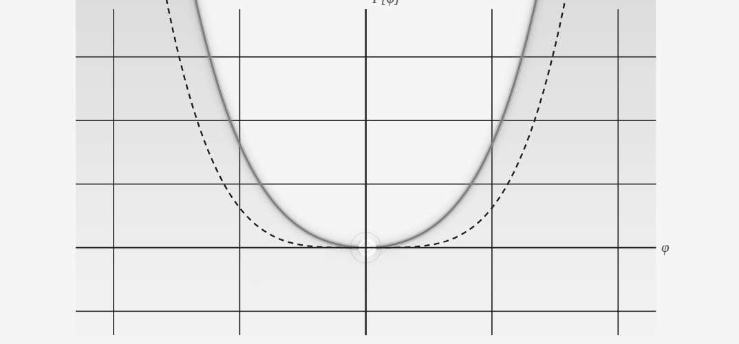
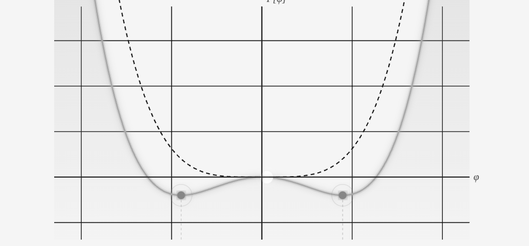
When $\varepsilon<0$ (below threshold, precausal) $\mathcal{F}$ has a unique minimum at $\psi=0$; when $\varepsilon>0$ (above threshold, instantiated) two symmetric minima appear at $\psi^{*}=\pm\sqrt{2\varepsilon}$. The full three-term structure of equation (23) is retained throughout the analysis.

The first term, $-\varepsilon(T(C))\,\psi^{2}$, governs the stability of the uninstantiated phase. The coefficient $-\varepsilon=\tau-|T(C)|$ changes sign at $|T(C)|=\tau$. When $|T(C)|<\tau$, $\varepsilon<0$ and this term increases $\mathcal{F}$ as $\psi$ increases from zero, keeping the uninstantiated state $\psi=0$ at a local minimum: configurations prefer to remain uninstantiated. When $|T(C)|>\tau$, $\varepsilon>0$ and the term now decreases $\mathcal{F}$ near $\psi=0$, destabilising the uninstantiated state and driving the configuration towards nonzero $\psi$. The sign change in $\varepsilon$ is precisely what defines the threshold.

The second term, $b\,\psi^{4}$ with $b>0$, is the quartic stabilisation term. Without it, the functional would be unbounded below for $T>\tau$, and $\psi$ could grow without limit. The quartic term ensures that once the uninstantiated phase becomes unstable, the configuration does not destabilise entirely but settles into a new, well-defined minimum at some finite value of $\psi$. It is this term that makes the transition a genuine phase change with a stable instantiated phase rather than a runaway.

The third term, $c\,|\nabla_{\mathcal{C}}\psi|^{2}$ with $c>0$, penalises inhomogeneity in $\psi$ across configuration space. If configurations with similar structures were to have very different modal statuses, the gradient would be large and the term would raise $\mathcal{F}$. This term is the formal analogue of the Ginzburg gradient term and has the physical effect of producing smooth, coherent transitions rather than discontinuous patches of instantiated and uninstantiated configurations. Its presence ensures that the transition is second order rather than first order, a point treated below.

This functional is structurally identical to the Landau–Ginzburg free energy of second order phase transitions [8], and the analogy is illuminating. In condensed matter physics, the Landau–Ginzburg functional describes how a system moves between phases as temperature changes. The order parameter tracks the degree of order (magnetisation, superconducting condensate, and so on), and the free energy determines which phase is stable at which temperature. In PST, the role of temperature is played by the asymmetric tension $T(C)$, the role of the order parameter is played by the modal status $\psi$, and the potential determines which mode of being, uninstantiated or instantiated, is stable at which tension level.

The difference from the condensed matter case is fundamental. In condensed matter, the phase transition is a dynamical process: it unfolds over time, involves fluctuations and nucleation, and is driven by thermal agitation. In PST, there is no temperature, no heat bath, no temporal evolution, and no dynamics. The transition is a modal reorganisation: a change in which mode of being is logically available to the configuration, not a change in the state of a system that exists in time. The Landau–Ginzburg structure is borrowed for its mathematical economy, not for its physical interpretation.

4.5.  Stability analysis and the two regimes

The most productive way to extract modal content from a functional is to identify which configurations minimise it. In classical mechanics, the principle of least action selects the physically realised trajectory from among all kinematically possible ones. In PST, the principle is modal rather than temporal: among all values of the order parameter available to a configuration of given tension $T(C)$, the modally self-consistent value is the one at which $\mathcal{F}$ attains its minimum. This is a variational statement, not a dynamical one. There is no time over which $\psi$ evolves towards its minimum; the minimum is the only modal position a configuration can coherently occupy given its tension. Configurations whose order parameter deviates from the minimum of $\mathcal{F}$ are modally incoherent: their degree of instantiation is inconsistent with the tension they carry.

The condition for a minimum is the vanishing of the first functional derivative, $\delta\mathcal{F}/\delta\psi=0$, the Euler–Lagrange condition [170] applied to the modal functional. Before writing the result, it is worth identifying the structural role of each term in $\mathcal{F}$. The quadratic term $-\varepsilon\langle\psi,\psi\rangle$ is the modal restoring term, and its sign change at the threshold is entirely responsible for the qualitative bifurcation in the behaviour of $\mathcal{F}$. The quartic term $b\langle\psi,\psi\rangle^{2}$ is the nonlinear saturation term: it is always positive and ensures the functional remains bounded below. The gradient term $c|\nabla_{\mathcal{C}}\psi|^{2}_{V_{7}}$ penalises rapid variation of $\psi$ across configuration space. Distributing $\delta/\delta\psi$ across these three terms and collecting, the modal equation of state is the $V_{7}$-vector equation:

$$-2\varepsilon\,\psi+4b\,\langle\psi,\psi\rangle\,\psi-2c\,\nabla_{\mathcal{C}}^{2}\psi=0$$ (25)

This equation has two qualitatively distinct regimes, separated by the threshold.

Below the threshold, $|T(C)|<\tau$: $\varepsilon<0$. The only solution to the uniform equation is $\psi=0\in V_{7}$. Since $\delta^{2}\mathcal{F}/\delta\psi^{2}\big{|}_{\psi=0}=-2\varepsilon\,\mathbb{1}_{V_{7}}>0$ (positive multiple of the identity), this is a local minimum in every direction of $V_{7}$. The configuration remains uninstantiated. This is the precausal phase.

Above the threshold, $|T(C)|>\tau$: $\varepsilon>0$. The solution $\psi=0$ is now a local maximum of $\mathcal{F}$ in every $V_{7}$-direction. The quadratic term falls with increasing $|\psi|$; the quartic term turns $\mathcal{F}$ upward again at large $|\psi|$. The result is a $G_{2}$-invariant Mexican-hat profile: a continuous family of degenerate minima at fixed radius, parameterised by the unit direction $\hat{\psi}\in S^{6}\subset V_{7}$.

The location of these minima requires explicit computation. Restricting to spatially uniform configurations, the equation of state reduces to $-2\varepsilon\,\psi+4b\,|\psi|^{2}\,\psi=0$, i.e. $2\psi\,(-\varepsilon+2b\,|\psi|^{2})=0$. The root $\psi=0$ is the maximum. The nontrivial roots satisfy $|\psi|^{2}=\varepsilon/(2b)$, giving the vacuum $6$-sphere

$$\mathcal{V} \;=\;\bigl{\{}\,\psi\in V_{7}\;:\;|\psi|=r_{0}\,\bigr{\}}\;\cong\;S^{6},$$ (26)

$$r_{0} =\sqrt{\frac{|T(C)|-\tau}{2b}}=\sqrt{\frac{\varepsilon(C)}{2b}}.$$

Modal sublimation locks $\hat{\psi}$ to the substrate-determined direction $\hat{\tau}=T(D)/|T(D)|$ on $\mathcal{V}$ (P2). The two “symmetric minima at $\psi=\pm r_{0}$” are the antipodal pair $\pm r_{0}\hat{\tau}$ in the 1-dim projection along $\hat{\tau}$; the full vacuum manifold has six tangent directions on $S^{6}$ orthogonal to $\hat{\tau}$, five of which, those perpendicular to the complex slice, carry the gauge-theoretic content (§14.2). The appearance of $\varepsilon(C)$ under the radical is structurally significant. The depth of instantiation, how far from zero the order parameter settles, is not a free parameter but is determined directly by how far the configuration’s tension sits above the threshold. A configuration with $\varepsilon$ barely positive instantiates shallowly; one deep in the instantiated regime carries a large order parameter. This relationship between excess tension and the degree of instantiation is one of the central quantitative predictions of PST.

There are two degenerate minima, symmetric about $\psi=0$. The configuration must occupy one of them, but the functional does not select which: both are equally deep. This is the instantiated phase. The two solutions correspond to the two structurally distinct orientations of the instantiated configuration, related by the symmetry $\psi\to-\psi$ that the functional possesses. That the functional carries this symmetry but the configuration that minimises it does not is the content of spontaneous symmetry breaking in the PST framework: the substrate selects a definite modal orientation without any external influence distinguishing the two options.

4.5.1.  Structural versus spontaneous asymmetry

PST has spontaneous symmetry breaking in the strict sense at the discrete $Z_{2}$ level: the $\psi\to-\psi$ symmetry of the functional is broken by the configuration’s choice of one of two equally-deep minima. In the richer complex-scalar formulation (and a fortiori the full $V_{7}$ formulation), the Landau–Ginzburg (LG) potential also carries a continuous symmetry. Its degenerate minima form a $\mathrm{U}(1)$ ring in the complex slice, and a $G_{2}$-orbit 6-sphere $\mathcal{V}\cong S^{6}\subset V_{7}$ in the full setting. In standard physics that would be the canonical spontaneous symmetry breaking (SSB) setup, producing Goldstone modes along $\mathcal{V}$.

PST departs from the standard SSB account at this angular level. P2’s asymmetric vector tension supplies a structural preferred direction $\hat{\tau}=T(D)/|T(D)|\neq 0$ in $V_{7}$ before any vacuum exists, and modal sublimation locks $\hat{\psi}$ to $\hat{\tau}$ by direct determination from the substrate’s directional bias (§1.7, P3 statement). The angular direction of the vacuum is therefore not a spontaneous choice: it is pinned by P2, upstream of the LG dynamics. What standard physics treats as a historical contingency (“which vacuum did the universe end up in?”) PST answers structurally: the substrate’s pre-existing tension direction selects it.

Two complementary readings of this layering, both correct:

1. PST inherits the SSB mathematics, sombrero potential, degenerate vacuum manifold, Goldstone modes, Higgs radial mode, the electroweak (EW) eaten Goldstones at the doublet level (§13.4), in full. The discrete $Z_{2}$ sign choice in the present paragraph is genuinely spontaneous.

2. PST redirects the spontaneous arbitrariness of the angular (continuous) direction: that selection is determined by P2, not by the SSB process. In standard-physics vocabulary the substrate’s structural asymmetry is closer to an explicit symmetry breaking term, except that the symmetry was never present in the substrate’s definition to begin with; P2 is not a perturbation added to a symmetric structure but a postulate of the substrate’s structure itself.

The asymmetry is therefore not derived away in PST: it is relocated from the spontaneous-arbitrary level (where standard physics leaves it) to the structural-postulate level (P2). Whether this is progress depends on whether one finds the postulate that the substrate’s tension functional is asymmetric under complementation more natural than a random vacuum selection at the SSB step.

One residue of spontaneity survives this relocation, and it is worth being exact about what it costs. The $Z_{2}$ choice between $+r_{0}\hat{\tau}$ and $-r_{0}\hat{\tau}$ is spontaneous in the standard sense: nothing upstream selects it. It is not, however, an openness of the same kind as the angular selection just removed. The modal potential is invariant under the full $G_{2}$ symmetry of $V_{7}$, and the involution $\psi\to-\psi$ is a $G_{2}$-equivariant special case of that invariance, as noted above. The two minima are therefore related by a symmetry of the entire structure in which they sit, so no quantity definable within that structure distinguishes them. There is no fact as to which sign was taken, and correspondingly nothing for the theory to explain: the residue is not an unanswered question but a question with no content.

The distinction is between two kinds of tie. A tie over whether any distinction obtains at all would be fatal, and it is precisely what the substrate’s asymmetry excludes: that is the balanced case, in which nothing is instantiated. A tie over which label an already-drawn distinction carries is harmless, because the distinction has been drawn and only the naming is undetermined. PST’s founding commitment rules out the first. It never undertook to rule out the second, and it does not need to.

The sign of $a$ is the fundamental discriminant between uninstantiated and instantiated existence. It is not a property of the configuration that can be read off directly; it is a property of the relationship between the configuration’s tension and the threshold. This is why the threshold is primary and the transition is a logical consequence, not a dynamical one.

4.6.  The bifurcation point and the derivation of $\tau$

The critical tension magnitude $\tau$ is the value at which the qualitative character of $\mathcal{F}$ changes: for $|T(C)|<\tau$, the uninstantiated phase $\psi=0\in V_{7}$ is the unique minimum; for $|T(C)|>\tau$, it is a maximum and a $6$-sphere of new minima appears. The moment of change is the bifurcation point, the magnitude of $T$ at which $\psi=0$ transitions from stable to unstable.

The characterisation of critical points as minima or maxima requires the second variation. For a $V_{7}$-valued field, the second functional derivative is a quadratic form on $V_{7}$ (a $7\times 7$ symmetric tensor). If the form is positive-definite, the functional is locally convex at $\psi_{0}$ in every $V_{7}$-direction; the configuration is at a stable minimum. If indefinite or negative-definite, at least one direction in $V_{7}$ is unstable.

The critical point of interest is $\psi=0$, the uninstantiated configuration. To determine whether this is modally stable (the precausal phase is robust) or unstable (it cannot be maintained), one must examine the curvature of $\mathcal{F}$ at this point. Restricting again to spatially uniform configurations ($\nabla_{\mathcal{C}}\psi=0$, the gradient term contributing only a non-negative Laplacian eigenvalue that does not affect the sign at $\psi=0$) and differentiating $\delta\mathcal{F}/\delta\psi=-2\varepsilon\psi+4b\,|\psi|^{2}\psi$ once more with respect to $\psi$ and evaluating at $\psi=0$ eliminates the cubic-in-$\psi$ terms entirely. What remains is purely the contribution of the quadratic term, proportional to the identity on $V_{7}$:

$$\frac{\delta^{2}\mathcal{F}}{\delta\psi^{2}}\bigg{|}_{\psi=0}=-2\varepsilon(|T|)\,\mathbb{1}_{V_{7}}=2\,(\tau-|T|)\,\mathbb{1}_{V_{7}}$$ (27)

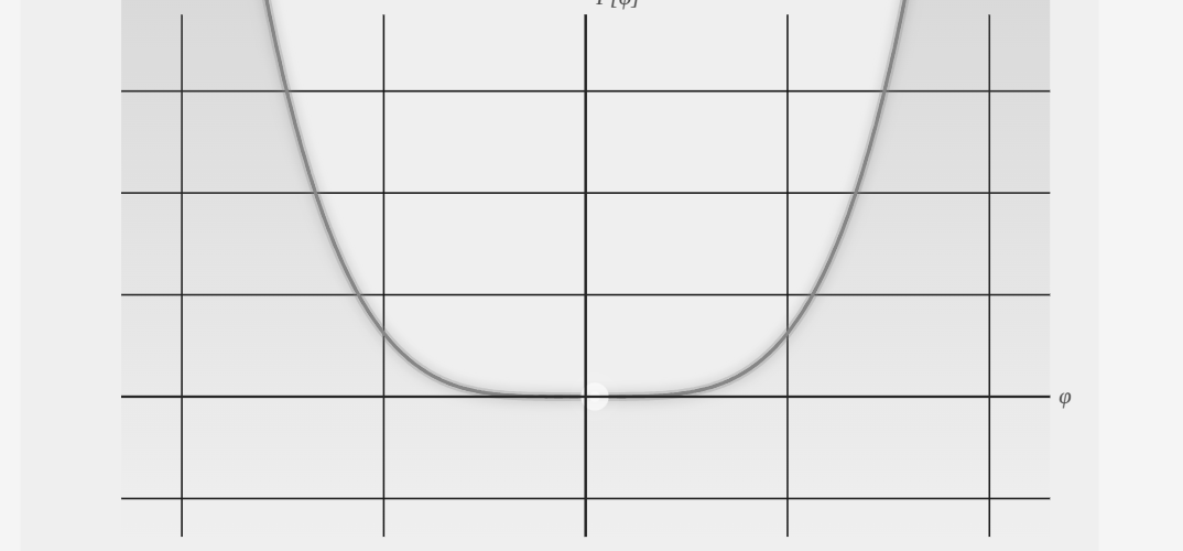
This is positive-definite for $|T|<\tau$ (i.e., $\varepsilon<0$), zero for $|T|=\tau$, and negative-definite for $|T|>\tau$ (i.e., $\varepsilon>0$). The $G_{2}$-isotropy of the second variation at $\psi=0$ is direct: the form is a scalar multiple of the identity, hence invariant under all $V_{7}$-rotations. The second variation vanishes at $T=\tau$, and this vanishing is the mathematical realisation of the threshold: the precise tension value at which the uninstantiated configuration ceases to be stable. What remains is to give $\tau$ a rigorous definition that does not presuppose its own value.

The naive approach would be to define $\tau$ as the solution to $\delta^{2}\mathcal{F}/\delta\psi^{2}\big{|}_{\psi=0}=0$, which from the expression above gives $-2\varepsilon=0$ and thus $|T|=\tau$, a circularity that conceals rather than reveals. The correct approach is to observe that $\tau$ is defined by a property of the functional, not by an algebraic equation: it is the magnitude below which $\psi=0$ is a stable minimum and above which it is not. This is precisely the infimum of the set of tension magnitudes for which the second variation vanishes:

$$\tau=\inf\left\{|T(C)|:\frac{\delta^{2}\mathcal{F}}{\delta\psi^{2}}\bigg{|}_{\psi=0}=0\right\}$$ (28)

The use of the infimum rather than a simple equation reflects the possibility that configurations at exactly $T=\tau$ form a set of measure zero in $\mathcal{C}$: the threshold is the greatest lower bound of all tension values that can trigger instantiation, and this bound may or may not be achieved by any individual configuration. In practice, when the functional takes the quadratic-quartic form above, the infimum is achieved and $\tau$ is well-defined as a specific value.

The significance of this derivation is that $\tau$ emerges from the structure of $\mathcal{F}$ itself. It is not a parameter that the theorist chooses. Once the functional is specified, its form constrained by the symmetries of the precausal substrate and the requirement that the transition be second order, the threshold is fixed. In this sense, the modal threshold is not a contingent feature of the theory. It is a structural necessity: any substrate governed by a modal potential of this form will have a threshold, and that threshold will be the bifurcation point of the functional.

4.6.1.  Notation: which threshold $\tau$ names

An unsubscripted $\tau$ means this threshold throughout the book: the modal threshold, a condition on the global tension $T(C)$ of a whole configuration. A decoration always signals something else. $\hat{\tau}\in S^{6}$ is the threshold direction that sublimation locks, a unit vector rather than a value. The null threshold $\tau_{\mathrm{null}}$ (§4.10) is a condition on the pairwise tension $T(\{a,b\})$, and it marks the causal boundary: the value at which a separation is null. It is the pairwise companion of $\tau$, determined jointly with it rather than posited independently. The outcome-dependent thresholds $\tau_{i}$ (§10.3) are the modal threshold shifted by a measurement coupling, one per available outcome. Where the text says “the threshold” with no qualifier, the modal threshold is meant.

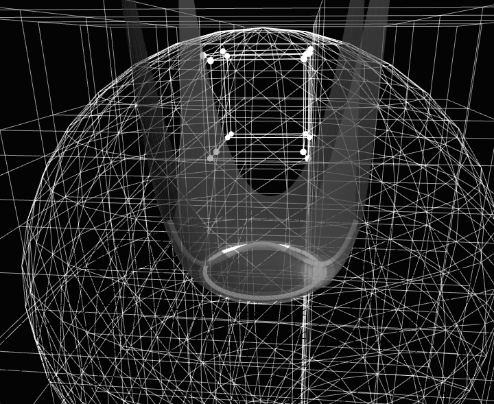
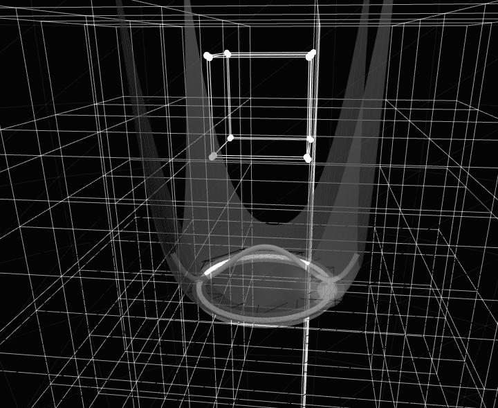
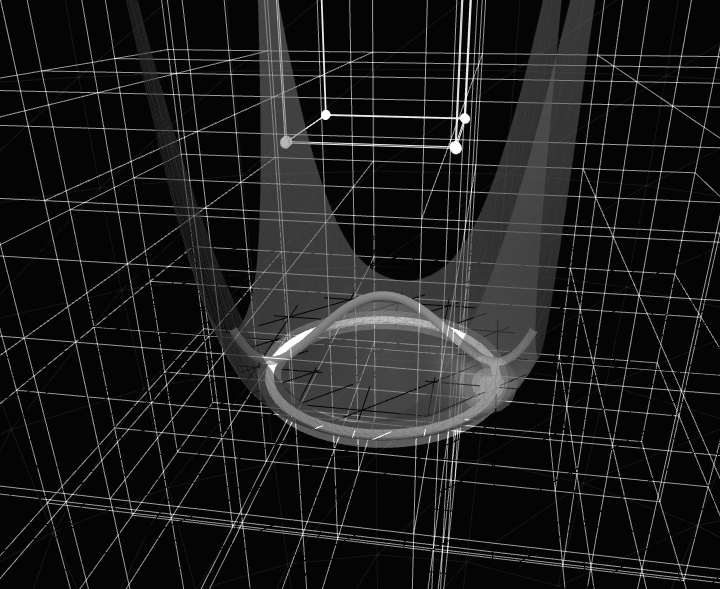
The passage from $\psi=0$ to the bifurcated minimum is modal sublimation, with no temporal unfolding. Figure 1 shows the modal potential on either side of the threshold and at it: a single valley below, the flattened critical point at $\varepsilon=0$, and the two degenerate minima above. §4.8 characterises that transition in detail.

Figure 1: The modal potential $F[\varphi]$ at three values of excess tension $\varepsilon$. Left: $\varepsilon={-}0.8$, single valley at $\varphi=0$; the substrate configuration rests at the unique minimum, uninstantiated. Centre: $\varepsilon=0$, the modal threshold; the valley flattens and the minimum is about to split. Right: $\varepsilon={+}0.8$, two degenerate minima at $\varphi=\pm\sqrt{\varepsilon}$ (the plotted curves use the rescaled variant $-\tfrac{1}{2}\varepsilon\,\varphi^{2}+\tfrac{1}{4}\varphi^{4}$; the canonical form of relation (1) below has minima at $\pm\sqrt{2\varepsilon}$); the configuration at $\varphi=0$ is now a local maximum and cannot remain there. The dashed curve is the reference potential at $\varepsilon=0$. The four key relations carried by this figure are: (1) the Landau–Ginzburg modal potential $F(\psi,\varepsilon)=-\varepsilon\,\langle\psi,\psi\rangle+\tfrac{1}{4}\langle\psi,\psi\rangle^{2}$ with quartic coefficient $b=\tfrac{1}{4}$ fixed by the LG form; (2) excess tension $\varepsilon=|T(\mathcal{C})|-\tau$; (3) the vacuum manifold radius $|\psi^{*}|=\sqrt{2\varepsilon}$ on $V_{7}$ with topology $\mathcal{V}\cong S^{6}$ (a 6-sphere of degenerate directions in $V_{7}$, projecting onto $S^{1}$ in any 2-plane slice of $V_{7}$); and (4) the projection map $\Phi:\mathcal{S}\to\mathcal{G}$ from the precausal substrate to instantiated geometry.

4.7.  Summary of the threshold half

Not every tension imbalance produces a universe. The threshold half of this chapter derives a critical tension value, the modal threshold $\tau$, below which the substrate remains abstract and unobservable, and above which it cannot remain that way. Think of water vapour: it can exist invisibly up to a certain temperature, but above that point it must condense. Below $\tau$, the configuration has a single stable resting state with no geometry; above $\tau$, that resting state becomes unstable and geometry must appear. The threshold is not assumed: it is calculated as the exact tension value at which the mathematical potential changes from single-welled to double-welled, and its existence is a structural necessity rather than a postulate.

The two postulates in play across this half are P2 (asymmetric vector tension, with $T(D)\neq 0$ in $V_{7}$ generically) and P3 (the $G_{2}$-invariant Landau–Ginzburg modal potential on $V_{7}$); from them follow the existence and value of the modal threshold $\tau$ as the bifurcation point of $F[\psi,\varepsilon]$ and the vacuum manifold $\mathcal{V}\cong S^{6}\subset V_{7}$ for $\varepsilon>0$. One point is worth disclosing explicitly: at the angular level the vacuum direction is not a spontaneous choice but is pinned by P2’s $\hat{\tau}$, while at the discrete $Z_{2}$ level the symmetry breaking is genuinely spontaneous in the standard sense; these layered roles are made explicit in the “structural versus spontaneous asymmetry” paragraph. The modelling choice is the $G_{2}$-invariant quartic functional form. The Bernoulli measure, under which $F$ is varied, is not a further choice: it is derived in §2.5 from per-property complementation invariance.

4.8.  The character of the threshold

What obtains at the modal threshold is unlike any physical process encountered in the instantiated world. It has no duration, no mechanism, no intermediate states, and no energy cost. It is not that it is very fast; temporal concepts simply do not apply to it. The precausal substrate is a nonspatiotemporal domain: there is no time in which a process could unfold, and no space across which it could propagate. What holds at the threshold is not a process but a modal reorganisation: a supra-threshold configuration is instantiated as geometry, where a sub-threshold one is not, and the two descriptions stand in this relation tenselessly.

Modal sublimation names this tenseless instantiation relation between the substrate description and the geometric description; it is not an event connecting two times. The substrate’s priority over geometry is logical and structural, not temporal: a supra-threshold configuration cannot remain uninstantiated by logical necessity (§17.8), and that logical priority, not a temporal one, is exactly what “precausal” means. Apparent processual language throughout this book, “crossing the threshold,” “the transition,” “the order parameter relaxes,” “the system settles”, is shorthand for that relation; no temporal process at the substrate level is implied.

The name sublimation is by analogy with the physical phenomenon in which a solid passes directly into a gaseous state, bypassing the liquid phase. In modal sublimation, every intermediate mode is bypassed because only two modes of being are available: uninstantiated existence within the precausal substrate, and instantiated existence as geometry. There is no intermediate mode that is partially spatial or partially causal.

Modal sublimation is characterised by four properties:

• Nontemporal: no before or after, no duration, no sequence of states; the configuration is instantiated with time, not located within a pre-existing time

• Nonmechanistic: no propagating influence, no force, no interaction

• Nonenergetic: no conservation law, no energy input or output

• Strictly modal: a change in the mode of being, not a change of state within an existing mode

Each of these four properties requires unpacking, because each contradicts a default assumption carried over from the instantiated world.

The nontemporal character is the most radical. In everyday physics, every process unfolds in time: there is a before and an after, a cause and an effect, a duration that can in principle be measured. Even processes described as instantaneous in non-relativistic mechanics, a collision, a decay, a measurement, are idealised limits of processes that have a finite, if arbitrarily small, duration. Modal sublimation is not a limit of this kind. It does not occur quickly; it does not occur in time at all. The configuration does not spend even an infinitesimal moment in transition. The reason is not dynamical but ontological: time is a structure of the instantiated domain, while instantiation is what constitutes that domain, not an event occurring within a prior time. To ask how long modal sublimation takes is to apply a concept to a context in which the concept has not yet been defined. This is not a failure of measurement precision; it is a logical impossibility of the same kind as asking what temperature a mathematical proof achieves. The configuration is not located within time; time is carried as a consequence of instantiation, not presupposed as a container in which a transition could unfold.

The nonmechanistic character follows directly from the nontemporal character. In the instantiated domain, every change of state is mediated by an interaction: a force, a field, a messenger particle, a propagating influence of some kind. These mediators all require spacetime in which to propagate and physical degrees of freedom to couple to. The precausal substrate has neither. No interaction can mediate the modal sublimation because interactions are structures of the domain that sublimation brings into being. There is no force that pushes a configuration across the threshold; the threshold is not a barrier that must be overcome but a logical boundary at which a particular mode of being ceases to be available. The transition is not driven by anything external. It is a logical consequence of the modal structure of the configuration itself, in the same way that the truth of a mathematical theorem is not caused by anything but follows necessarily from the axioms. This has a crucial implication: PST does not require a mechanism, an initial impetus, or a first cause. The demand for a mechanism is itself an instantiated-world concept, and applying it to the transition that precedes instantiation is a category error of the same kind as the causal question discussed in Chapter 5.

The nonenergetic character removes the last temptation to treat modal sublimation as a physical event in disguise. Energy is a conserved quantity defined within the instantiated domain: it requires a Hamiltonian, a time-translation symmetry via Noether’s theorem [21], and ultimately a spacetime manifold on which these structures can be defined. None of these are available in the precausal substrate. The relevant conservation statement in PST is not energetic but modal: it is the preservation of the asymmetric tension functional $T(C)$ across the threshold. The tension that characterises the precausal configuration is the same quantity that, after projection via $\Pi$, appears as the stress-energy tensor $T_{\mu\nu}$ in the instantiated domain, as shown in Chapter 7. The Einstein field equations, on this reading, are not equations of motion governing a physical process; they are a conservation statement expressing that the structural content of the precausal configuration is faithfully preserved in the instantiated geometry. Nothing is created across the threshold; nothing is destroyed. The same structural content is expressed in a different modal register, the way that the same logical argument can be expressed in different formal languages without gaining or losing content.

The strictly modal character is the most philosophically precise formulation of what the other three properties imply. A change of state within an existing mode, a particle moving, a field oscillating, a temperature rising, leaves the mode of being intact while altering something within it. The ontological register is unchanged: the system is still a physical system in spacetime, governed by the same causal laws, measured in the same units. Modal sublimation changes the mode itself. The configuration does not acquire new properties within the precausal substrate; it changes the ontological register in which all its properties are expressed. Before sublimation, the configuration’s structural content exists as modal tension in a nonspatiotemporal domain. After sublimation, that same structural content exists as geometric curvature and matter-energy in a Lorentzian manifold. There is no moment at which the configuration is partially in each mode; the two modes stand in a strictly modal relation, not a temporal one, even though the phrasings “before” and “after” used here strictly apply only after time has come into being. This is the precise sense in which PST’s fundamental relation is irreducible to any physical process: physical processes are changes of state within the instantiated mode, while modal sublimation is the relation that constitutes the mode itself, not a happening within it.

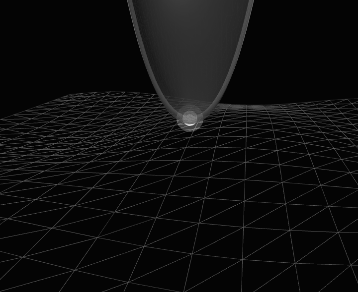
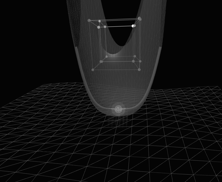
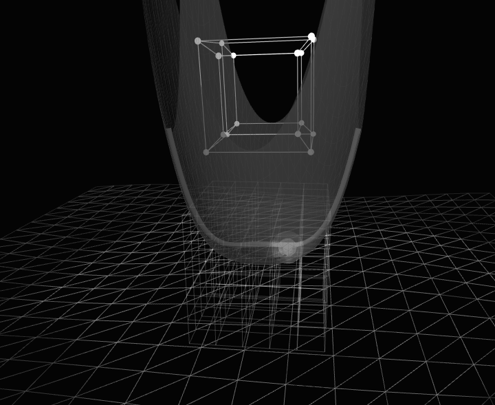
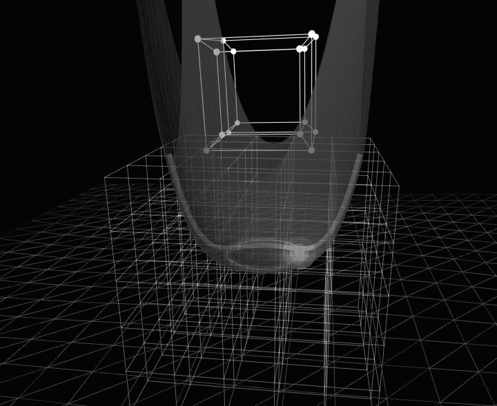
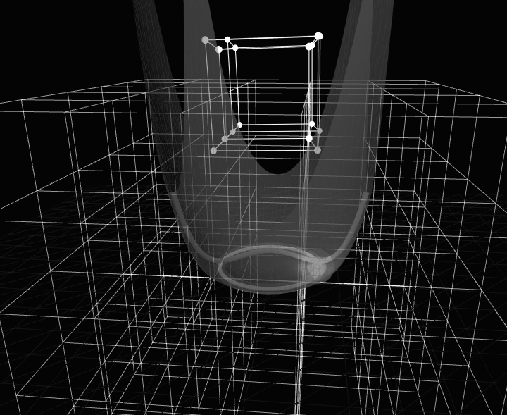
The result of this transition is a geometry: a Lorentzian manifold $(M,g)$ that becomes the spacetime background for all subsequent physical processes. Geometry does not emerge within spacetime; it becomes spacetime in the act of sublimation. Figure 2 traces the whole passage across eight values of the excess tension $\varepsilon$, from the precausal bowl to the degenerate vacuum manifold.

$\varepsilon={-}1.00$	$\varepsilon=0$	$\varepsilon={+}0.15$	$\varepsilon={+}0.30$
$\varepsilon={+}0.50$	$\varepsilon={+}0.70$	$\varepsilon={+}0.90$	$\varepsilon={+}1.00$

Figure 2: Visual model of modal sublimation across eight values of the excess tension $\varepsilon=|T(C)|-\tau$ (§4.6): $\varepsilon<0$ precausal, $\varepsilon\geq 0$ instantiated. Sampling is dense on the instantiated side, where the geometric content emerges; a single precausal reference frame at $\varepsilon={-}1.00$ shows the pre-threshold state from which everything else unfolds. Each frame shows the modal potential $F[\psi,\varepsilon]=-\varepsilon\psi^{2}+\tfrac{1}{4}\psi^{4}$ rendered as a rotationally symmetric surface (lower portion), with the bright tube tracing its one-dimensional cross-section and the white sphere marking the position of the order parameter $\psi$ at the current potential minimum. Top-left frame ($\varepsilon={-}1.00$): the precausal substrate; the potential forms a deep bowl with a single minimum at $\psi=0$, the order parameter is confined to the origin, and a flat proto-manifold grid is shown for reference. Threshold and early instantiation ($\varepsilon=0$ to $\varepsilon\approx{+}0.30$): the bowl flattens and its centre rises, the high-dimensional cube descends towards the bowl, the spacetime lattice crystallises, and the ring of minima begins to form at the base. Mid to deep instantiation ($\varepsilon\approx{+}0.50$ to ${+}1.00$): the potential has acquired a continuous 6-sphere of degenerate minima (the vacuum manifold $\mathcal{V}\cong S^{6}\subset V_{7}$); the figure displays the 2-plane projection visible as a bright ring $\mathcal{V}_{\hat{\eta}}\cong S^{1}$ in any $\hat{\tau}$-perpendicular slice; the spatial slice closes, shown by the $S^{3}$ dome enveloping the local chart; and the finite internal factor $A_{F}=\mathbb{C}\oplus\mathbb{H}\oplus M_{3}(\mathbb{C})$ consolidates as the cube snaps onto the spacetime grid.

4.9.  Categorical formulation: the sublimation functor

The mathematical language suited to a transition between fundamentally different types of structure is category theory, specifically the theory of functors between categories [9]. Construct two categories as follows. The precausal category $\mathbf{S}$ has as objects all configurations $C\in\mathcal{C}$ with $T(C)\geq\tau$, and as morphisms distinction preserving maps $f:C\rightarrow C^{\prime}$. The geometric category $\mathbf{G}$ has as objects Lorentzian manifolds $(M,g)$ and as morphisms smooth maps preserving the causal structure.

Modal sublimation is the functor:

$$\Phi:\mathbf{S}\rightarrow\mathbf{G}$$ (29)

with four properties encoding the fundamental features of the transition:

1. $\Phi$ exists at the categorical boundary; it is not a morphism within $\mathbf{S}$ or $\mathbf{G}$, formalising the nonmechanistic character of the transition

2. $\Phi$ carries tension into geometry: the pairwise tensions fix the metric $g$ of the instantiated manifold via equation (30), and the tension projection $\Pi$ (equation (32)) supplies the stress-energy $T^{(\mathrm{iso})}_{\mu\nu}$; scalar curvature then follows from $g$ through the field equations of Chapter 7

3. $\Phi$ is surjective: every Lorentzian manifold arises as the image of some precausal configuration

4. $\Phi$ has no inverse: once a configuration is instantiated, the geometric domain has no access to the precausal substrate that produced it

4.10.  Explicit construction of $\Phi$

The projection functor $\Phi$ inherits the post-sublimation directional structure of the substrate: it is constructed relative to the $\hat{\tau}$-direction that modal sublimation locks (P2). The construction below produces a spacetime $M$ and a realisation $\rho$ together with an internal-factor identification along $\hat{\tau}$; the same construction at a different $\hat{\tau}^{\prime}\in S^{6}$ would produce a $G_{2}$-rotated copy of the same $\Phi$, with the rotation an unphysical relabelling. Once $\hat{\tau}$ is fixed by the substrate’s directional bias, $\Phi$ is determined up to the gauge freedom described below.

The functor is constructed in three steps.

Step 1, Geometric realisation. The manifold $M$ and the map $\rho$ are not given independently before the construction; they are jointly determined by it.

A legitimate concern requires attention before the construction proceeds. The notation $\rho:D\rightarrow M$ appears to presuppose $M$, a set of spacetime points, before the construction that is supposed to produce spacetime has been carried out. If spacetime points are already available as the target of $\rho$, then the theory has not derived spacetime from the substrate; it has merely labelled pre-existing points with properties from $D$. This would be a foundational circularity.

The resolution is that $M$ is not given prior to and independently of $\rho$. The construction proceeds in the following order. First, note that any surjective function $\rho:D\twoheadrightarrow X$, for any set $X$, partitions $D$ into equivalence classes: $a\sim_{\rho}b$ if and only if $\rho(a)=\rho(b)$. The equivalence classes $[a]_{\rho}=\{b\in D:\rho(b)=\rho(a)\}$ are the fibres of $\rho$, and their collection $D/{\sim_{\rho}}$ is a quotient set that depends only on $D$ and the partition, not on any property of $X$. A spacetime point is then defined to be a fibre of $\rho$: it is an equivalence class of properties, not a pre-existing geometric entity. The manifold $M$ is the quotient set $D/{\sim_{\rho}}$ equipped with whatever additional structure (topology, differentiable structure, metric) the subsequent steps impose. The map $\rho$ is thus a quotient map, and $M$ is a derived set: it comes into existence as the image of $\rho$, rather than being a container that $\rho$ maps $D$ into.

This construction has a philosophical precedent in Leibniz’s principle of the identity of indiscernibles: things that share all the same properties are the same thing. Here, the converse is operative, properties that are assigned to the same geometric locus by $\rho$ are identified, and the locus is nothing over and above that identification. A spacetime point has no content beyond the property-bundle it collects; it is not an additional ontological entity.

More concretely: $M$ is characterised as any smooth manifold of dimension $n$ whose topology and differential structure are consistent, a posteriori, with requiring that the metric constructed in Step 2 is well-defined and smooth. Among all candidate manifolds satisfying this consistency condition, the tension structure of $(D,\delta)$ further constrains which are admissible: a candidate $M$ is admissible if and only if there exists a partition of $D$ whose induced tension structure $T(\{[a],[b]\})=T(\{a,b\})$ reproduces the relational data already present in $(D,\delta)$. This constraint, not an external stipulation, selects the spacetime topology and dimension.

Given a choice of admissible $M$, define the realisation map $\rho:D\rightarrow M$ as the quotient projection sending each property $a\in D$ to its equivalence class $\rho(a)=[a]_{\rho}\in M$. The nonuniqueness of $\rho$, the freedom to partition $D$ into fibres in multiple ways that are all consistent with the tension structure, is precisely the diffeomorphism invariance of General Relativity [1, 10]. It emerges here as a consequence of the nonuniqueness of geometric realisation from the pre-geometric substrate, rather than as a separately imposed symmetry. There is no canonical labelling of spacetime points: this is not a deficiency of the theory but a structural result, matching the gauge freedom of general relativity (GR).

Step 2, Tension-to-metric map. Introduce the null threshold $\tau_{\mathrm{null}}\in\mathbb{R}^{+}$ as the pairwise-tension companion of $\tau$, determined jointly with $\tau$ rather than posited as an independent input. While $\tau$ is a condition on the global tension $T(C)$, $\tau_{\mathrm{null}}$ is a condition on pairwise tensions $T(\{a,b\})$: it is the value at which the two-property tension is null, i.e., at which $g=0$ by definition. The two thresholds operate at different levels. Their relationship reduces to the same input as the rate-integral computation of §16.7: an explicit form of the global tension functional $T(C)$ as a functional of the pairwise tensions $T(\{a,b\})$ at the postulate level, which the canonical form fixes up to the configuration’s content (§19.9.1). Once the explicit functional is specified, $\tau$ is the critical value of $T(C)$ at which the modal potential loses its single-well stability (§4.1) and $\tau_{\mathrm{null}}$ is its pairwise restriction; the two are then determined jointly, not independently. The metric is then:

$$g_{\mu\nu}\!\left(\rho(a),\rho(b)\right)=\eta_{\mu\nu}\cdot\operatorname{sgn}\!\left(\tau_{\mathrm{null}}-T(\{a,b\})\right)\cdot\left|T(\{a,b\})-\tau_{\mathrm{null}}\right|^{1/2}$$ (30)

where $\eta_{\mu\nu}$ is a placeholder for the diagonal sign pattern $\mathrm{diag}(+1,-1,-1,-1)$ that the construction induces, not a presupposition of Minkowski geometry. Its appearance here is definitional. The signature theorem below shows that the sign pattern is fixed, downstream of the tension structure, by hyperbolic well-posedness of the Goldstone wave equation, and $\eta_{\mu\nu}$ names that pattern: the mostly-minus signature $(+,-,-,-)$ used throughout. The Clifford convention is $\gamma_{0}^{2}=+I$, $\gamma_{i}^{2}=-I$, giving the local Dirac algebra $\mathrm{Cl}(1,3)\cong M_{2}(\mathbb{H})$ (Chapter 13). This gives:

• $T(\{a,b\})=\tau_{\mathrm{null}}\;\Rightarrow\;g=0$: null separation

• $T(\{a,b\})>\tau_{\mathrm{null}}\;\Rightarrow\;g<0$: spacelike

• $T(\{a,b\})<\tau_{\mathrm{null}}\;\Rightarrow\;g>0$: timelike

The Lorentzian signature is forced as a theorem by hyperbolic well-posedness of the Goldstone wave equation (Computation 2, §4.12): the Cauchy problem for $\Box_{g}\theta=0$ admits a well-posed initial-value formulation and a conserved Noether current only for signature $(1,n-1)$. The bifurcation of tension values around $\tau_{\mathrm{null}}$ remains the algebraic mechanism inside the LG variational structure; what Computation 2 shows is that the sign cut required for that bifurcation is not an independent axiom but a consequence of the well-posedness condition.

Two clarifications are necessary. First, equation (30) is strictly a pairwise assignment: it attaches a signed scalar to each pair of realised points, not a $(0,2)$-tensor to a tangent space. The metric tensor field $g_{\mu\nu}(x)$ is recovered by the continuum limit: take $a$ and $b$ to be nearby properties such that $\rho(a)$ and $\rho(b)$ approach $x$ along a tangent vector $v^{\mu}$; then $g_{\mu\nu}(x)\,v^{\mu}v^{\nu}$ arises as the limit of equation (30) along the chord, analogous to recovering a Riemannian metric as the Hessian of a distance function. Second, the magnitude $\bigl{|}T(\{a,b\})-\tau_{\mathrm{null}}\bigr{|}^{1/2}$ is the minimal-regularity choice. A linear dependence would give a metric with a non-smooth gradient at the null cone, while the square root yields Hölder-$\tfrac{1}{2}$ behaviour there. That is the appropriate regularity class for a structure that degenerates at $T=\tau_{\mathrm{null}}$, and it ensures that equation (109) blows up precisely at the modal null threshold rather than at $T=0$.

Step 3, Action on morphisms. For $f:C\rightarrow C^{\prime}$ in $\mathbf{S}$, $\Phi(f):(M,g)\rightarrow(M^{\prime},g^{\prime})$ is the diffeomorphism induced by $f$ via $\rho$. Distinction preserving maps in $\mathbf{S}$ correspond precisely to causal structure preserving maps in $\mathbf{G}$, ensuring functoriality.

The projection operator. Define the tension projection operator $\Pi$:

$$\Pi(T(C))(x)=\int_{\mathcal{C}}T(C^{\prime})\cdot K(x,C^{\prime})\,d\mu(C^{\prime})$$ (31)

where $K(x,C^{\prime})=\delta(x-\rho(C^{\prime}))$ for local configurations. The role of $\Pi$ here is structurally analogous to the Dirac operator in Connes’ noncommutative geometry [48]: in both cases a single operator bridges an underlying non-spatial structure to the instantiated domain (the metric itself is supplied by $\Phi/\rho$, not by $\Pi$). The stress-energy tensor at $x\in M$ in the isotropic, homogeneous case is:

$$T^{(\mathrm{iso})}_{\mu\nu}(x)=\Pi(T(C))(x)\cdot g_{\mu\nu}(x)$$ (32)

This scalar form $T^{(\mathrm{iso})}_{\mu\nu}=\Pi(T(C))\,g_{\mu\nu}$ gives a stress-energy tensor proportional to the metric, which is the correct structure for a cosmological constant ($T_{\mu\nu}=\Lambda g_{\mu\nu}$) but not for general matter distributions. Two facts fix its scope exactly, and they are narrower than “isotropic” (Computation 155). Applying the Bianchi identity to $T_{\mu\nu}=\Pi\,g_{\mu\nu}$ gives $\nabla^{\mu}T_{\mu\nu}=\partial_{\nu}\Pi$, so conservation forces $\Pi$ to be constant; and a perfect fluid is proportional to $g_{\mu\nu}$ if and only if $\rho+p=0$, i.e. $w=-1$. So the scalar form is not the leading-order approximation for isotropic sources: an isotropic dust or radiation fluid is already outside it. It is exactly and only the cosmological constant. The general form requires $\Pi$ to be a tensor-valued projection $T_{\mu\nu}(x)=\Pi_{\mu\nu}(T(C))(x)$, whose components encode the directional distribution of tension in the precausal configuration. §7.4 supplies its structure, the mechanism that sets the equation of state, and the weight itself, which is fixed by requiring the tensor and scalar projections to agree (§7.4.4). The noninvertibility of $\Phi$ is immediate: $\rho$ discards the internal structure of $D$ that does not affect pairwise tensions. Geometry encodes the projection of $T$ through $\Pi$ but not the full precausal configuration that generated it, just as a shadow records an object’s outline but not its internal structure.

4.11.  Uniqueness of $\Phi$ and the origin of diffeomorphism invariance

The construction proceeds via an explicit choice of realisation map $\rho:D\rightarrow M$, which is not determined by the precausal structure alone. This raises the question of how strongly the output functor $\Phi$ depends on the choice of $\rho$, and what that dependence implies for the physical content of the theory. The answer is a uniqueness theorem: $\Phi$ is unique up to diffeomorphism, and the ambiguity in $\Phi$ is completely and exactly characterised by diffeomorphism invariance, with no residual freedom beyond it.

The proof follows directly from the construction. Given $\rho$, the metric $g_{\mu\nu}$ at every pair of points is fully determined by equation (30): there are no further choices once the realisation map is fixed. Now suppose $\rho^{\prime}=f\circ\rho$ for some smooth bijection $f:M\rightarrow M^{\prime}$. The tension values $T(\{a,b\})$ depend only on $a,b\in D$, not on their images under $\rho$, so they are unchanged by the substitution. Therefore the metric computed at $(\rho^{\prime}(a),\rho^{\prime}(b))$ via equation (30) satisfies $g^{\prime}(\rho^{\prime}(a),\rho^{\prime}(b))=g(\rho(a),\rho(b))$, which is exactly the condition that $(M^{\prime},g^{\prime})$ is the pushforward of $(M,g)$ along $f$. Any two choices of $\rho$ therefore produce Lorentzian manifolds that are diffeomorphic to one another, together with a corresponding natural isomorphism between the two functors they define. $\Phi$ is unique up to this natural isomorphism, which at the level of manifolds is a diffeomorphism.

What the uniqueness theorem leaves open is not a further gauge choice but which substrate configuration is instantiated: the realisation map $\rho$ is fixed up to diffeomorphism once the configuration is given, but the theory must still say which configuration sublimation realises. P3 supplies this through maximum entropy: modal sublimation instantiates the $\mu$-typical (maximum-entropy) configuration, not a $\mu$-exceptional one. The permutation symmetry of the substrate measure already forces equidistribution in measure; maximum-entropy sublimation strengthens this to the realised configuration itself, so its emergence cloud $\rho_{n}$ is metric-covariantly equidistributed at the closure rate $\eta_{K,R}<d_{0}^{2}/4$. This is exactly condition A3 of the Mosco limit (§18.1); it therefore holds as a consequence of P3, and the Mosco convergence to $M=\mathbb{R}\times S^{3}$ closes under A1–A7, A3 being supplied by P3 rather than assumed (§18.1). The selection is a typicality principle internal to P3, the analogue of maximum-entropy or generic-initial-data selection elsewhere in physics: it adds no fourth postulate and derives no rate from more primitive structure, but it locates the equidistribution where it belongs, in the dynamics of instantiation.

The physical significance of this result is that diffeomorphism invariance in General Relativity is not an additional symmetry requirement that must be imposed upon the theory by hand. It is the complete characterisation of the non-uniqueness of $\Phi$: the relabelling freedom in choosing $\rho$ survives into the instantiated manifold as coordinate freedom, and coordinate freedom is diffeomorphism invariance. There is no finer ambiguity and no coarser one; the two are identical, which is the uniqueness theorem stated at the head of this section.

A note on the metric signature. The argument in Step 2 assigned the Minkowski signature $(+,-,-,-)$ through equation (30), by bifurcating pairwise tensions about a null threshold $\tau_{\mathrm{null}}$ that separates spacelike from timelike separations. This determines the signature given $\tau_{\mathrm{null}}$: once a sign cut is supplied, $T>\tau_{\mathrm{null}}$ is spacelike and $T<\tau_{\mathrm{null}}$ is timelike, by construction. It does not determine that exactly one direction lies below $\tau_{\mathrm{null}}$. Spectral asymmetry of the tension spectrum about a threshold, whose standard form is $T(C)\neq T(\bar{C})$, complement-asymmetry, is consistent with zero, one, or several eigenvalues lying below any given cut, so it does not by itself fix the count of timelike directions. Any $S_{D}$-invariant Gram construction over real features is positive-semidefinite by elementary linear algebra, so the negative eigenvalue required for one timelike direction cannot arise from $S_{D}$-symmetry alone. It must be supplied by an indefinite bilinear form beyond the Gram construction. The Lorentzian signature $(+,-,-,-)$ is fixed as a theorem via Computation 2 of §4.12: hyperbolic well-posedness of the Goldstone wave equation forces $(p,q)=(1,n-1)$, and the $\mathrm{U}(1)$ Noether-current conservation that produces the angular-momentum identification requires this same Lorentzian signature. The macroscopic dimension $n=4$ that combines with the signature to give the four-dimensional Lorentzian spacetime $M=\mathbb{R}\times S^{3}$ follows from real K-theory (KO) additivity given the verified spectral-triple structure (§1.5): the substrate’s parity-selected KO-6 (Computation 3) and the product’s KO-2 mod 8 (Connes Lorentzian value) together force $M$ at KO-dimension four. PST is then the theory that derives everything downstream from $(D,\delta)$ + LG + the realisation map $\rho$, with both signature and macroscopic dimension outputs rather than inputs.

4.12.  Lorentzian signature from Goldstone hyperbolic well-posedness

This section makes self-contained the result that Lorentzian signature follows from hyperbolic well-posedness of the Goldstone wave equation (Computation 2): we state the partial differential equation (PDE), the function spaces, the energy estimate, and show why one timelike direction (signature $(p,q)=(1,n-1)$) is the unique signature compatible with a well-posed Cauchy problem on the projected spacetime $\mathbb{R}\times S^{3}$.

The logical order forestalls any apparent circularity. The manifold $M=\mathbb{R}\times S^{3}$ and its differentiable structure emerge first, as the Mosco limit of the Boolean Dirichlet form (§7.8), carrying a topology but as yet no metric signature; the signature is then fixed downstream as the unique one for which the Goldstone wave equation on that already-emergent manifold admits a well-posed Cauchy problem. Hyperbolicity does not presuppose a metric, it selects among the candidate signatures available on a manifold that exists prior to any of them.

The PDE. After modal sublimation has selected the vacuum manifold $\mathcal{V}\cong S^{6}\subset V_{7}$ (§1.7, P3), the Goldstone phase $\theta$ along the broken direction satisfies, at the quadratic order of the LG functional, the second-order PDE

$$g^{\mu\nu}\,\partial_{\mu}\partial_{\nu}\,\theta(x)\;=\;0,\qquad x\in M,\;\;\mu,\nu=0,1,\ldots,n-1,$$ (33)

where $g^{\mu\nu}$ is the (Wick-rotation-undetermined) [161] signature-$(p,q)$ metric on $M=\mathbb{R}\times S^{3}$ obtained as the projection of the LG kinetic term to emergent spacetime. The order parameter contributes $r_{0}^{2}|\nabla\theta|^{2}$ to the LG free energy, which under $\nabla\to g^{\mu\nu}\partial_{\mu}\otimes\partial_{\nu}$ becomes the wave operator.

A note on which degree of freedom this is. (33) is written massless, as the Goldstone mode of a spontaneously broken symmetry is. The order parameter’s angular directions are not that: P2 supplies $\hat{\tau}$ before any vacuum exists and modal sublimation determines $\hat{\psi}$ from it (§4), so those six directions are constrained rather than dynamical, and the residual $\mathfrak{so}(6)$ fixes the vacuum and is therefore unbroken. Neither yields a Goldstone (Computation 170). What carries $\theta$ is the phase: $\hat{\tau}$ is a real direction in $V_{7}$ and determination fixes a direction while saying nothing about a phase, so the complex line $\mathbb{C}\hat{\tau}$ survives the constraint where the real line does not, and the phase of the complexified order parameter is left free (Computation 171). It is exactly massless whenever the couplings to $\hat{\tau}$ are phase-blind, which gauge invariance enforces, since $\mathrm{Re}\langle\psi,\hat{\tau}\rangle$ is not invariant under $\psi\mapsto\mathrm{e}^{i\alpha}\psi$ while the moduli are. That makes the complex-valued order parameter a requirement rather than the richer of two formulations: a real one has no phase and so no $\theta$, and with no $\theta$ the signature theorem loses the mode it argues from. What does not depend on the answer is everything below: Hadamard well-posedness is decided by the principal symbol $g^{\mu\nu}\xi_{\mu}\xi_{\nu}$, so even a massive $\theta$ would leave the argument untouched. The signature theorem needs hyperbolicity, not masslessness, and is more robust than its original statement claimed (Computation 170).

Cauchy problem and function spaces. The Cauchy problem for equation (33) on the time slice $\Sigma_{0}=\{0\}\times S^{3}$ asks: given initial data $(\theta_{0},\theta_{1})\in H^{1}(S^{3})\times L^{2}(S^{3})$, does there exist a unique solution $\theta\in C(\mathbb{R};H^{1}(S^{3}))\cap C^{1}(\mathbb{R};L^{2}(S^{3}))$ with $\theta|_{\Sigma_{0}}=\theta_{0}$, $\partial_{t}\theta|_{\Sigma_{0}}=\theta_{1}$?

For the Cauchy problem to be well-posed in the Hadamard sense [110] (existence, uniqueness, and continuous dependence on initial data) the principal symbol $g^{\mu\nu}\xi_{\mu}\xi_{\nu}$ of equation (33) must be strictly hyperbolic with respect to the splitting $\Sigma_{0}$, i.e. the polynomial

$$g^{00}\omega^{2}\;+\;2g^{0i}\omega\xi_{i}\;+\;g^{ij}\xi_{i}\xi_{j}\;=\;0$$ (34)

must have exactly two real roots $\omega=\omega_{\pm}(\xi)$ for every nonzero spatial covector $\xi\in T^{*}\Sigma_{0}$ [99]. Strict hyperbolicity forces the metric to have one timelike direction (transverse to $\Sigma_{0}$) and $n-1$ spacelike directions. Equivalently, signature $(p,q)=(1,n-1)$ (or its sign-reversal $(n-1,1)$, the same content).

Energy estimate. Given strict hyperbolicity, multiplying equation (33) by $\partial_{t}\theta$ and integrating over $\Sigma_{t}$ yields the standard wave energy

$$E(t)\;=\;\tfrac{1}{2}\int_{\Sigma_{t}}\bigl{(}\,(\partial_{t}\theta)^{2}\;+\;g^{ij}\partial_{i}\theta\,\partial_{j}\theta\,\bigr{)}\sqrt{g_{S^{3}}}\,dx$$ (35)

which is conserved: $E(t)=E(0)$ for all $t\in\mathbb{R}$. Energy conservation immediately gives existence (via the standard semigroup construction [99]), uniqueness (the zero-data Cauchy problem has zero energy and hence zero solution by Gronwall), and continuous dependence (initial-data perturbations propagate at finite speed bounded by $\max|g^{ij}/g^{00}|^{1/2}$ along light cones). This is the standard Sobolev-space well-posedness theory for the wave equation [99].

What fails in other signatures. Three alternatives must be considered and ruled out:

1. Euclidean $(p,q)=(0,n)$. All directions are spacelike; the principal symbol $g^{\mu\nu}\xi_{\mu}\xi_{\nu}$ is positive-definite. Equation (33) becomes elliptic (Laplace) rather than hyperbolic. The Cauchy problem for an elliptic equation is famously ill-posed (Hadamard’s classical example [110]): small perturbations in the data give exponentially growing perturbations in the solution, so no continuous-dependence map exists. Modal sublimation produces a domain that admits time evolution, not an elliptic boundary-value problem; Euclidean signature is therefore incompatible with the Cauchy-problem structure of modal sublimation.

2. Ultra-hyperbolic $(p,q)$ with $p\geq 2$, $q\geq 2$. Two or more timelike directions. The principal symbol has signature $(p,q)$ as a quadratic form, but the Cauchy problem on the codimension-$p$ “time” submanifold has multiple time derivatives in the data, and strict hyperbolicity in the sense above fails: the polynomial in $\omega$ has either no real roots (for some $\xi$) or more than two. The Cauchy problem is ill-posed in the Hadamard sense; existence fails for generic smooth data [111, 112].

3. $(p,q)=(n,0)$ (anti-Lorentzian). All directions timelike, no spatial direction. Equation (33) has no propagation direction; the projection has no instantiated geometry to speak of. Excluded as a degenerate case.

Conclusion. The unique signature compatible with a well-posed Cauchy problem for the Goldstone wave equation on the Mosco-limit spacetime $M=\mathbb{R}\times S^{3}$ is $(p,q)=(1,n-1)$. Combined with the $n=4$ fix from the minimal KO-split (§1.5), this gives $(p,q)=(1,3)$, i.e. signature $(+,-,-,-)$. Lorentzian signature is therefore a theorem of modal sublimation rather than an additional postulate: the directionality of the threshold crossing selects time, hyperbolic well-posedness selects the number of spatial directions, and Computation 2 classifies the admissible signatures symbolically by the principal symbol of the free wave operator, beside its Derrick scaling table.

The above is a structural derivation using standard PDE theory [99]; the energy estimate is rigorous and the alternative-signature arguments are sketched at standard textbook level rather than fully worked. A fully rigorous treatment with detailed Sobolev-space analysis is straightforward but would expand this section substantially; the structural conclusion does not depend on which level of analytic detail one prefers. Computation 2 carries the symbolic signature classification; the energy estimate itself is standard and is not reproduced there.

4.13.  Summary

Modal sublimation is the moment the threshold is crossed, not a moment in time, but a logical transition. When a configuration’s tension exceeds $\tau$, it cannot remain in its abstract precausal state; it is compelled, by the same kind of necessity that makes a mathematical theorem true, to become concrete. The result is a four-dimensional spacetime with the Lorentzian signature that physics recognises. This section constructs the map from the precausal domain to the geometric domain, shows it is unique, and proves that the coordinate-freedom of General Relativity (diffeomorphism invariance) is a consequence of that uniqueness rather than a separate postulate.

Concretely, the modal-sublimation functor $\Phi:\mathcal{S}\to\mathcal{G}$ is constructed explicitly in three steps. Its central derived result (Computation 2) is that hyperbolic well-posedness of the Goldstone wave equation along $\hat{\tau}$ forces the Lorentzian signature $(+,-,-,-)$. The energy-estimate and PDE details are sketched here, with the energy estimate itself standard and not reproduced in full. The sign cut at $\tau_{\mathrm{null}}$, where hyperbolicity flips, exists because that well-posedness requirement demands it, not because it is posited; its value is determined jointly with $\tau$ through the explicit form of $T(C)$, the same explicit form the rate integral of §16.7 awaits, so the joint determination is not yet carried out. Diffeomorphism invariance is likewise derived, from the non-uniqueness of the realisation map $\rho$. The passage $\mathcal{S}\to M=\mathbb{R}\times S^{3}$ is a theorem under A1–A7, resting on Mosco convergence of the Boolean Dirichlet form to the Laplace–Beltrami form on $M$. The argument is structural, and is stated explicitly in §18.1 with seven assumptions A1–A7. Equicoercivity A7 is itself a theorem given A1, A2, A4 and A3 of §18.1.6, which combines a standard Poincaré inequality with the equidistribution condition A3, a uniform-rate hypothesis on $H^{1}$-bounded compactly-supported test functions, supplied by P3’s maximum-entropy sublimation. A3 is corroborated for the i.i.d. surrogate (Computation 70), which confirms the rate P3 supplies for the emergence-determined cloud. The minimal KO-split $4+6=10$ given the KO-$6$ substrate (§1.5) fixes $n=4$, and is not a selection: KO-dimension is additive and the admissible pair is unique, so there is nothing to minimise over (§1.5, Computation 148).